Foreword

This document has been prepared by the OpenEAC Alliance, a collaborative group of energy engineering and measurement and verification professionals focused on creating transparent and standardized methods to measure the environmental impacts of demand side interventions. These methodologies are designed to align with best practices and reflect input from industry experts. The OpenEAC Alliance aims to enhance accountability and consistency in documenting energy and carbon savings from distributed energy resources (DERs).

About the OpenEAC Alliance

The OpenEAC Alliance is an organization of professionals dedicated to standardizing the measurement and verification of DERs. By focusing on clarity and rigor, the Alliance aims to overcome challenges that have hindered the proper valuation of DERs for their climate benefits. Central to this effort is the Energy Attribute Certificate (EAC), a standard that provides a detailed, auditable record of energy project impacts, including attributes such as type, timing, and location of energy production or reduction.

The OpenEAC Alliance collaborates to develop open-source methodologies, ensuring that DER projects can be accurately measured, verified, and valued in a way that promotes trust and drives market adoption.

Introduction

This document introduces a standardized approach for quantifying energy and carbon savings achieved through electrification interventions for the purposes of generating Energy Attribute Certificates (EACs). The approach utilizes a comprehensive building energy dataset to estimate the energy and carbon impacts of electrification initiatives. This dataset offers detailed building-level energy insights, which can be scaled based on project characteristics to quantify hourly changes in fuel and electricity emissions.

Scope

This document outlines the methodology, assumptions, and data sources used to quantify energy and carbon savings from electrification interventions based on device-level temperature and flow rate data. The primary purpose is to specify how quantified changes in energy use and emissions avoidance can be translated into Energy Attribute Certificates (EACs).

Scope: The purpose of this methodology is to estimate the device-level savings from the fuel-switching component (use of heat) from a combined heat pump space and water heating device that contains water temperature and flow rate sensors. This device may also contain an auxiliary heating and cooling unit.

Normative References

The following documents are essential for the application of this specification. For references with no date, the latest edition applies:

• NEEA Heat Pump Water Heater Field Study Report

Terms and Definitions

• Legacy System

  • UEFlegacy (Uniform Energy Factor): A measure of the efficiency of the legacy system’s water heater.

  • AFUE (Annual Fuel Utilization Efficiency): A measure of the heating efficiency of the legacy system’s furnace or boiler.

  • SEER2 (Seasonal Energy Efficiency Ratio 2): A measure of the cooling efficiency of the legacy system’s air conditioner or heat pump.

  • HSPF2 (Heating Seasonal Performance Factor 2): A measure of the heating efficiency of the legacy system’s heat pump.

  • Water Heater Rated Storage Volume (gallons): The quantity in gallons that the legacy water heater system can hold (N/A if tankless)

• Heat TimeSeries Fields

  • Qdhw: Total energy delivered from heat pump for domestic hot water

  • Qheat: Total energy delivered to hydronic coil

• Electricity Timeseries Fields

  • System

    • ehpwh: Electrical energy used by heat pump water heater to generate hot water

    • ebooster: Electrical energy used by electric booster (if applicable)

    • ecirc: Electrical energy used by circulation pump for hydronic heating

    • efan-hydro: Electrical energy used by fan during hydronic heating

    • efan-heat: Electrical energy used by fan during DX heating

  • Auxiliary System

    • eaux-heat: Electrical energy used by heat pump AC for heating

    • eaux-cool: Electrical energy used for cooling

    • efan-aux-cool: Electrical energy used by fan during cooling

  • Other

    • efan-only: Electrical energy used by fan when in fan mode

    • eelec: Electrical energy used by electronics

• Water TimeSeries Fields

  • galdhw: gallons of water used for domestic hot water purposes

  • galheat: gallons of water used for hydronic space heating

Methodology

1 Impact Calculation

1.1 Calculate hourly observed electricity energy consumption based on the average hourly power drawn per hour.

1.1.1 Sum all electricity signals that can be associated with the device.

1.2 Calculate counterfactual domestic hot water avoided energy device-level consumption:

1.2.1 Calculate the average hourly heat output for domestic hot water (QDHW)

1.2.1.1 Calculate the difference in temperature between the cold water entering the tank and the hot water pre-mix valve. Multiply this by the flow rate of water into the tank and the weight of water in order to get the energy required to heat the water. Take the average of all of the readings and multiply by 60 to get the hourly energy output.

1.2.1.1.1 $\displaystyle Q_{dhw}(t) = (T_1(t) - T_2(t)) \cdot \dot{DF}_1(t) \cdot 8.34$

1.2.1.1.2 $\displaystyle Q^{(h)}_{dhw} = \frac{1}{N}\sum_{t=1}^{N} Q_{dhw}(t) \cdot 60$

1.2.2 Calculate the required energy (in BTUs) that would be required to produce QDHW. In the following equations, the energy source can be either electricity or gas, and all BTUs are associated with the energy source of the counterfactual system.

1.2.2.1 Tankless (energy source can be electricity or gas)

1.2.2.1.1 BTUenergy-source-water = Qdhw / UEF

1.2.2.2 Gas Storage

1.2.2.2.1 BTUenergy-source-water = Qdhw / (demandBasedEfficiency(UEFlegacy, galDHW)

1.2.2.2.1.1 See Section 2 for demandBasedEfficiency explanation

1.2.2.3 Gas Combined

1.2.2.3.1 BTUenergy-source-water = Qdhw+Qheat / (demandBasedEfficiency(UEF, galDHW+galheat)

1.2.2.3.1.1 See Section 2 for demandBasedEfficiency explanation

1.2.2.4 Electric Resistance

1.2.2.4.1 BTUenergy-source-water = Qdhw / (demandBasedEfficiency(UEFlegacy, galDHW)

1.2.2.4.1.1 See Section 3 for demandBasedEfficiency explanation

1.2.2.5 Electric Heat Pump

1.2.2.5.1 BTUenergy-source-water = Qdhw / (demandBasedEfficiency(UEFlegacy, galDHW)

1.2.2.5.1.1 See Section 4 for demandBasedEfficiency explanation

1.3 Calculate counterfactual space heating avoided energy device-level consumption:

1.3.1 Calculate the average hourly heat output for space heating (Qheat)

1.3.1.1 For space heating, calculate the difference in temperature between the heating return water to the tank and the water sent to the hydronic coil. Multiply this by the flow rate of water into the hydronic coil and the weight of water in order to get the energy required to heat the water. Take the average of all of the readings and multiply by 60 to get the hourly energy output.

1.3.1.1.1 $\displaystyle Q_{heat}(t) = (T_1(t) - T_3(t)) \cdot \dot{DF}_2(t) \cdot 8.34$

1.3.1.1.2 $\displaystyle Q^{(h)}_{heat} = \frac{1}{N}\sum_{t=1}^{N} Q_{heat}(t) \cdot 60$

1.3.2 Calculate the required energy (in BTUs) that would be required to produce Qheat

1.3.2.1 Gas Furnace or Gas Boiler

1.3.2.1.1 BTUgas-space = (Qheat+Qaux-heat) / AFUE

1.3.2.1.2 BTUelec-space = efan-hydro + efan-aux-heat

1.3.2.2 Gas Combined

1.3.2.2.1 BTU = 0

1.3.2.2.1.1 Assume that all BTUs are calculated in Section 1.2.2.2.

1.3.2.3 Electric Resistance

1.3.2.3.1 BTUelec-space = Qheat + Qaux-heat

1.3.2.4 Electric Furnace or Electric Boiler

1.3.2.4.1 BTUelec-space=efan-hydro+efan-aux-heat+(Qheat+Qaux-heat)/AFUE

1.3.2.5 Electric Heat Pump

1.3.2.5.1 BTUelec-space=(Qheat+Qaux-heat)/HSPF2

1.4 Calculate counterfactual fan and auxiliary cooling avoided energy device-level consumption

1.4.1 Calculate the average hourly heat output for auxiliary cooling (Qaux-cool).

1.4.2 Calculate the energy (in BTUs) that would be required to produce Qaux-cool. Also include any fan-only electrical consumption.

1.4.2.1 If a SEER2 value was provided

1.4.2.1.1 BTUelec-other=efan-only+(Qaux-cool/SEER2)

1.4.2.2 Otherwise

1.4.2.2.1 BTUelec-other=eaux-cool+efan-aux-cool

1.5 Sum the counterfactual BTUs for each energy source and convert them to their base units to get the counterfactual energy consumption:

1.5.1 Counterfactualelec-wh = (BTUelec-water+BTUelec-space+BTUelec-other) * 1 Wh / 3.412 BTUs

1.5.2 Counterfactualgas-wh = (BTUgas-water+BTUgas-space) * 1 Therm / 100,000 BTUs

1.6 Subtract the observed electricity consumption from the counterfactual electricity consumption in order to get the net electricity impact. The negative of the counterfactual gas consumption is the net gas impact.

2 Demand-Based Efficiency Calculation Methods for Water Heaters

2.1 Logarithmic Regression of Federal Regulations (10 CFR 430.32(d)(1)) energy conservation standards for central air conditioners and heat pumps.

2.1.1 The following assumption is made regarding the relationship between Draw Patterns and daily/hourly draw rates:

2.1.1.1 Very small: 10 gallons/day = 0.42 gallons/hr

2.1.1.2 Low: 38 gallons/day = 1.58 gallons/hr

2.1.1.3 Medium: 55 gallons/day = 2.29 gallons/hr

2.1.1.4 High: 84 gallons/day = 3.5 gallons/hr

2.1.2 Steps

2.1.2.1 Calculate the UEF for each draw pattern based on the legacy systems rated storage volume

2.1.2.2 Run a logarithmic regression on the gallons/hr vs UEF in order to estimate the efficiency of that system at different draw rates.

2.1.2.3 Rescale this logarithmic regression by the ratio between the legacy system’s rated UEF and the minimum efficiency standard UEF for a system of that rated storage volume and draw pattern (UEF/UEFmin)

2.1.2.4 Use this regression as the function in $\displaystyle \text{demandEfficiencyRescaleFactor} = \frac{\text{UEF}}{\text{UEF}{\min}}\left(X_0 + X_1 \cdot \ln(\text{gal}_{\text{dhw}} + \text{gal}_{\text{heat}})\right)$, but bound the result so that the minimum factor is 0.25 and the maximum factor is 0.8.

Appendix

Appendix 1: Federal Regulations energy conservation standards

The following table comes from the Code of Federal Regulations (10 CFR 430.32(d)(1)) which specifies minimum Uniform Energy Factor (UEF) standards for residential water heaters manufactured before May 6, 2029 for Gas-fired Storage Water Heaters and Electric Water Heaters.

Gas-fired Storage Water Heaters

Rated Storage Volume and Input Rating (if applicable)	Draw Pattern	Uniform Energy Factor (Vr is rated storage volume in gallons)
20<=X<=55	Very Small	0.3456 - (0.0020 * Vr)
	Low	0.5982 - (0.0019 * Vr)
	Medium	0.6483 - (0.0017 * Vr)
	High	0.6920 - (0.0013 * Vr)
55<X<=100	Very Small	0.6470 - (0.0006 * Vr)
	Low	0.7689 - (0.0005 * Vr)
	Medium	0.7897 - (0.0004 * Vr)
	High	0.8072 - (0.0003 * Vr)

For the Electric Water Heaters, based on the estimated UEFs, we assume that the 20<X<55 rated storage formulas are for electric resistance and the larger volume is for heat pumps.

Electric Storage Water Heaters

Rated Storage Volume and Input Rating (if applicable)	Draw Pattern	Uniform Energy Factor (Vr is rated storage volume in gallons)
20<=X<=55	Very Small	0.8808 - (0.0008 * Vr)
	Low	0.9254 - (0.0003 * Vr)
	Medium	0.9307 - (0.0002 * Vr)
	High	0.9349 - (0.0001 * Vr)
55<X<=120	Very Small	1.9236 - (0.0011 * Vr)
	Low	2.0440 - (0.0011 * Vr)
	Medium	2.1171 - (0.0011 * Vr)
	High	2.2418 - (0.0011 * Vr)

Appendix 2: Example of Demand-Based Efficiency Rescale Factor Calculation for Gas-Fired Water Heater

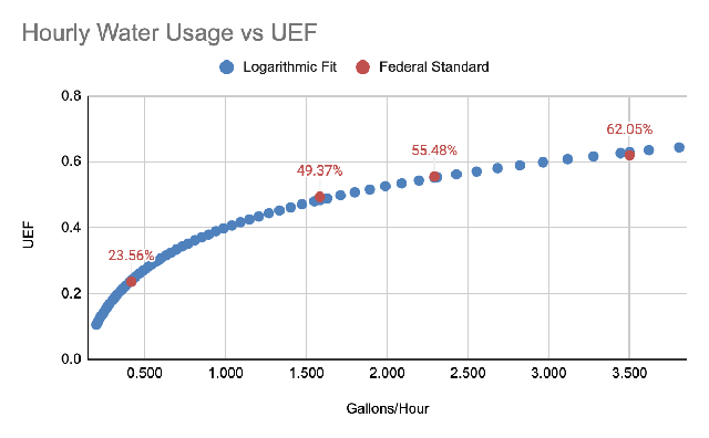
1 Using a legacy High Draw Pattern with a rated storage volume of 50 gallons and UEF of 0.68 and the table in Appendix 1, calculate the UEF:

Draw pattern	Estimated Gallons/day (gpd)	Estimated Gallons/hour (gph)	Calculated UEF for a 50 gallon tank
Very small	10	0.42	25%
Low	38	1.58	50%
Medium	55	2.29	56%
High	84	3.50	63%

2 Run a logarithmic regression on gallons/hour vs UEF achieves the following results:

Parameters	Value
a (intercept)	0.400000
b (slope)	0.182900
R²	0.998912
Equation	y = 0.4 + 0.1829*ln(gph)

3 Rescale with the rated UEF to get the resulting equation, bounded for very small and very large draw patterns:

$\displaystyle \text{demandBasedEfficiency} = \frac{0.68}{0.63} \times (0.4 + 0.1829 \times \ln(\text{gph})), \quad \text{bounded by } [0.25,\ 0.8]$

Appendix 3: Example of Demand-Based Efficiency Rescale Factor Calculation for Electric Resistance Water Heater

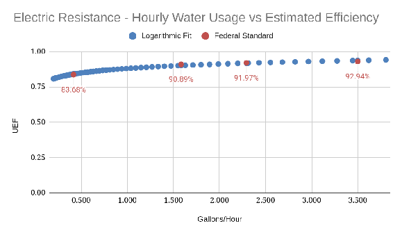
1 Using a legacy High Draw Pattern with a rated storage volume of 50 gallons and UEF of 0.95 and the table in Appendix 1, calculate the UEF:

Draw pattern	Estimated Gallons/day (gpd)	Estimated Gallons/hour (gph)	Calculated UEF for a 50 gallon tank
Very small	10	0.42	84%
Low	38	1.58	91%
Medium	55	2.29	92%
High	84	3.50	93%

2 Run a logarithmic regression on gallons/hour vs UEF achieves the following results:

Parameters	Value
a (intercept)	0.8799
b (slope)	0.0452
R²	0.9744
Equation	y = 0.8799 + 0.0452*ln(gph)

3 Rescale with the rated UEF to get the resulting equation, bounded for very small and very large draw patterns:

$\displaystyle \text{demandBasedEfficiency} = \frac{0.95}{0.93} \times (0.8799 + 0.0452 \times \ln(\text{gph})), \quad \text{bounded by } [0.84,\ 1]$

Appendix 4: Demand-Based Efficiency Rescale Factor Calculation for Electric Heat Pump Water Heaters

The electric heat pump water heater (HPWH) follows the same demand-based efficiency construction as the gas example in Appendix 2 — calculate a UEF per draw pattern, fit a logarithmic regression of gallons/hour against UEF, then rescale — with three differences specific to heat pumps, described below.

For a heat pump, the Uniform Energy Factor is greater than 1 and is equivalent to a coefficient of performance (COP): the device delivers more thermal energy than the electricity it consumes. The federal minimum standards for electric heat pumps top out near a UEF of ~2.0, which understates modern HPWH performance, so the rescaling step (Step 3) targets a field-supported COP rather than the legacy rated UEF.

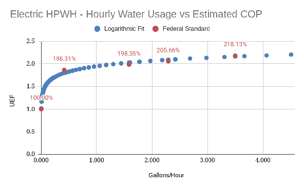
1 Calculate the COP for each draw pattern, and anchor the curve at zero draw.

Using the federal electric heat pump standards (the >55 gallon class) for a 50-gallon tank, the COP for each draw pattern is:

Draw pattern	Estimated Gallons/day (gpd)	Estimated Gallons/hour (gph)	Calculated COP for a 50 gallon tank
None	0.1	0.004	100%
Very small	10	0.42	186%
Low	38	1.58	198%
Medium	55	2.29	206%
High	84	3.50	218%

In addition to the four federal draw patterns, we add a zero-draw anchor: at negligible demand the device provides no demand-based gain, so its efficiency reverts to 100% (COP = 1.0). Because the logarithmic form is undefined at exactly zero, “zero” draw is represented by a near-zero rate of 0.1 gpd. This anchor sets the low-demand behavior of the curve and is the heat pump analogue of the very-small-draw bound used for gas.

2 Run a logarithmic regression on gallons/hour vs COP, which achieves the following results:

Parameters	Value
a (intercept)	1.946800
b (slope)	0.170200
R²	0.9914
Equation	y = 1.9468 + 0.1702 · ln(gph)

3 Rescale with the rated UEF to get the resulting equation but apply a 0.75 derating factor, because manufacturer UEFs (3.5–4.0) overstate real annual COP — field studies put modern HPWHs closer to 2.5–3.0. The 0.75 factor brings a 4.0 UEF unit to roughly a 3.0 COP, in line with observed field performance. Bound the output by 1.0 and the derated UEF.

$\displaystyle \text{demandBasedEfficiency} = \frac{\text{UEF}}{2.18} \times 0.75 \times \big(1.9468 + 0.1702 \cdot \ln(\text{gph})\big), \quad \text{bounded by } [1.0,\ \text{UEF} \times 0.75]$